# Validate in independent part, named gustoB
# main effects
lrm.val.full <- predict(full, newdata = gustoB, type = "lp")
# simple interaction
lrm.val.int1 <- predict(fullints, newdata = gustoB, type = "lp")
# Plot
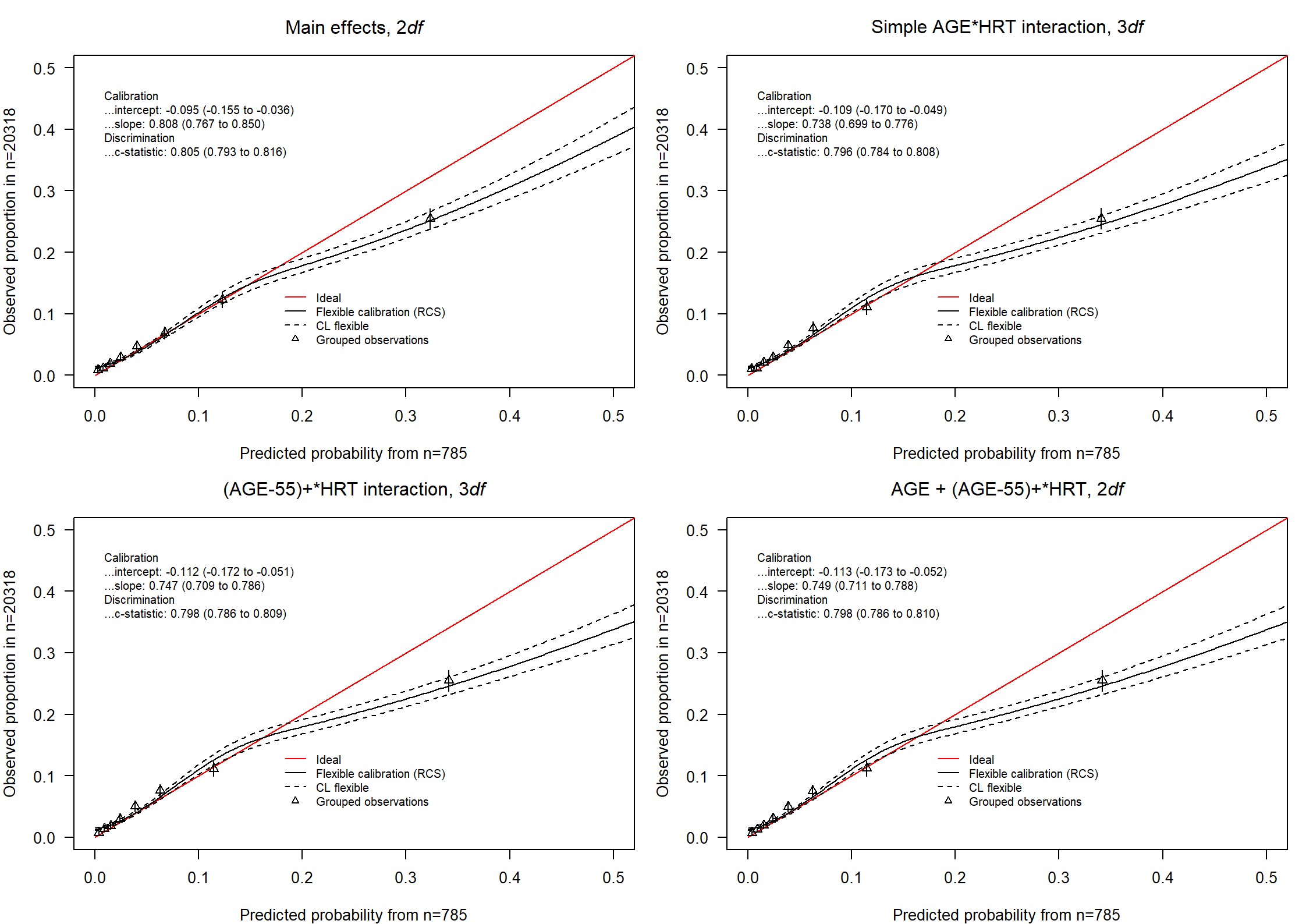
val.prob.ci.2(
y = gustoB[, "DAY30"], logit = lrm.val.full, riskdist = "predicted", logistic.cal = F,
smooth = "rcs", nr.knots = 3, g = 8, xlim = c(0, .5), ylim = c(0, .5),
legendloc = c(0.18, 0.15), statloc = c(0, .4), roundstats = 3,
xlab = "Predicted probability from n=785", ylab = "Observed proportion in n=20318"
)