7  Missing values

Figure and Table 7.1

###################################
# Ewout Steyerberg, Aug 18, 2018 #
# Missing values: illustrate MCAR, MAR, MNAR mechanism
# Use simple linear models
###################################

library(rms) # Harrell's library with many useful functions

#########################

set.seed(1) # For identical results at repetition
n <- 10000 # arbitrary, large, sample size
# n <- 1000000           # used for book

x2 <- rnorm(n = n, mean = 0, sd = 1) # x2 standard normal
x1 <- rnorm(n = n, mean = 0, sd = 1) # Uncorrelated x1
# x1   <- sqrt(.5) * x2 + rnorm(n=n, mean=0, sd=sqrt(1-.5))  # x2 correlated with x1

y1 <- 1 * x1 + 1 * x2 + rnorm(n = n, mean = 0, sd = sqrt(1 - 0)) # generate y
# var of y1 larger with correlated x1 - x2

plot(x = x1, y = x2, pch = ".", xlim = c(-4, 4), ylim = c(-4, 4), ps = .1)
abline(ols(x2 ~ x1))

# Make approx half missing
# x1: MCAR, MAR and MNAR mechanisms
x1MCAR <- ifelse(runif(n) < .5, x1, NA) # MCAR mechanism for 50% of x1
x1MARx <- ifelse(rnorm(n = n, sd = .8) < x2, x1, NA) # MAR on x2, R2 50%, 50% missing (since mean x2==0)
x1MARy <- ifelse(rnorm(n = n, sd = (sqrt(3) * .8)) > y1, x1, NA) # MAR on y, R2 50%, 50% missing (since mean y1==0)
x1MNAR <- ifelse(rnorm(n = n, sd = .8) < x1, x1, NA) # MNAR on x1, R2 50%, 50% missing (since mean x1==0)

# y1: MCAR, MAR and MNAR mechanisms
yMCAR <- ifelse(runif(n) < .5, y1, NA) # MCAR mechanism for 50% of x1
yMARx2 <- ifelse(rnorm(n = n, sd = .8) < x2, y1, NA) # MAR on x2, R2 39%, 50% missing (since mean x2==0)
yMNAR <- ifelse(rnorm(n = n, sd = .8) < y1, y1, NA) # MNAR on x1, R2 50%, 50% missing (since mean x1==0)

## Correlations ##
cor(is.na(x1MCAR), x2)^2

[1] 8.531179e-05

cor(is.na(x1MARx), x2)^2

[1] 0.3922284

cor(is.na(x1MARy), y1)^2

[1] 0.3905377

cor(is.na(x1MNAR), x1)^2

[1] 0.3909611

# y
cor(is.na(yMCAR), y1)^2

[1] 1.549048e-08

cor(is.na(yMARx2), x2)^2

[1] 0.3924581

cor(is.na(yMNAR), y1)^2

[1] 0.5305992

# End check correlations; 0.388 for those with some correlation, 0.52 for yMNAR

### Fig 7.1 ###
### Examine relation between x1 and x2
par(pty = "s")
# MCAR
plot(x = x1[1:500], y = x2[1:500], pch = 4, xlim = c(-4, 4), ylim = c(-4, 4), cex = 1.2, xlab = "x1", ylab = "x2", col = "darkgreen") # Orig
abline(ols(x2 ~ x1), lty = 2, lwd = 2, col = "darkgreen")
points(x = x1MCAR[1:500], y = x2[1:500], pch = "o", col = "red") # MCAR
abline(ols(x2 ~ x1MCAR), lty = 1, lwd = 2, col = "red")
title("a=0, b=0", cex.main = 2)

# x1MARx
plot(x = x1[1:500], y = x2[1:500], pch = 4, xlim = c(-4, 4), ylim = c(-4, 4), cex = 1.2, xlab = "x1", ylab = "x2", col = "darkgreen") # Orig
abline(ols(x2 ~ x1), lty = 2, col = "darkgreen")
points(x = x1MARx[1:500], y = x2[1:500], pch = "o", col = "red") # MCAR
abline(ols(x2 ~ x1MARx), lty = 1, lwd = 2, col = "red")
title("a=0.6, b=0", cex.main = 2)

# x1MARy
plot(x = x1[1:500], y = x2[1:500], pch = 4, xlim = c(-4, 4), ylim = c(-4, 4), cex = 1.2, xlab = "x1", ylab = "x2", col = "darkgreen") # Orig
abline(ols(x2 ~ x1), lty = 2, col = "darkgreen")
points(x = x1MARy[1:500], y = x2[1:500], pch = "o", col = "red") # MCAR
abline(ols(x2 ~ x1MARy), lty = 1, lwd = 2, col = "red")
title("a=-0.4, b=-0.1", cex.main = 2) # -.413, -.149

# x1MNAR
plot(x = x1[1:500], y = x2[1:500], pch = 4, xlim = c(-4, 4), ylim = c(-4, 4), cex = 1.2, xlab = "x1", ylab = "x2", col = "darkgreen") # Orig
abline(ols(x2 ~ x1), lty = 2, col = "darkgreen")
points(x = x1MNAR[1:500], y = x2[1:500], pch = "o", col = "red") # MCAR
abline(ols(x2 ~ x1MNAR), lty = 1, lwd = 2, col = "red")
title("a=0, b=0", cex.main = 2)

## y ##
# y MCAR
plot(x = x1[1:500], y = x2[1:500], pch = 4, xlim = c(-4, 4), ylim = c(-4, 4), cex = 1.2, xlab = "x1", ylab = "x2", col = "darkgreen") # Orig
abline(ols(x2 ~ x1), lty = 2, col = "darkgreen")
points(x = x1[!is.na(yMCAR)][1:250], y = x2[!is.na(yMCAR)][1:250], pch = "o", col = "red") # yMCAR
abline(ols(x2[!is.na(yMCAR)][1:10000] ~ x1[!is.na(yMCAR)][1:10000]), lty = 1, lwd = 2, col = "red")
title("a=0, b=0", cex.main = 2)

# y MAR
plot(x = x1[1:500], y = x2[1:500], pch = 4, xlim = c(-4, 4), ylim = c(-4, 4), cex = 1.2, xlab = "x1", ylab = "x2", col = "darkgreen") # Orig
abline(ols(x2 ~ x1), lty = 2, col = "darkgreen")
points(x = x1[!is.na(yMARx2)][1:250], y = x2[!is.na(yMARx2)][1:250], pch = "o", col = "red") # yMCAR
abline(ols(x2[!is.na(yMARx2)][1:10000] ~ x1[!is.na(yMARx2)][1:10000]), lty = 1, lwd = 2, col = "red")
title("a=0.6, b=0", cex.main = 2)

# y MNAR
plot(x = x1[1:500], y = x2[1:500], pch = 4, xlim = c(-4, 4), ylim = c(-4, 4), cex = 1.2, xlab = "x1", ylab = "x2", col = "darkgreen") # Orig
abline(ols(x2 ~ x1), lty = 2, col = "darkgreen")
points(x = x1[!is.na(yMNAR)][1:250], y = x2[!is.na(yMNAR)][1:250], pch = "o", col = "red") # yMCAR
abline(ols(x2[!is.na(yMNAR)][1:10000] ~ x1[!is.na(yMNAR)][1:10000]), lty = 1, lwd = 2, col = "red")
title("a=0.5, b=0.2", cex.main = 2)

### End Fig 7.1 ###

## Table 7.1 ##
mean(x1MARy, na.rm = T)

[1] -0.3579431

mean(x2[!is.na(x1MARy)], na.rm = T)

[1] -0.3703634

mean(x1MNAR, na.rm = T)

[1] 0.6202571

# y MNAR
mean(yMNAR, na.rm = T)

[1] 1.266413

mean(x1[!is.na(yMNAR)], na.rm = T)

[1] 0.4039278

mean(x2[!is.na(yMNAR)], na.rm = T)

[1] 0.4216802

Figure 7.2

## Fig 7.2 ##

############################################################
## Make plot function for graphs with y~x1; 4 with y~x2 ##
## First for missing x1, then missing y
############################################################

refx1 <- ols(y1 ~ x1)
refx2 <- ols(y1 ~ x2)
nsel <- 500

CCplot <- function(x1, y1, sel, reffit, lab, xlab = "x", ylab = "y", nsel1 = 400, nsel2 = 200, nsel3 = 800) {
  par(pty = "s")
  plot(x = x1[1:nsel], y = y1[1:nsel], pch = 3, xlim = c(-4, 4), ylim = c(-6, 6), cex = 1.2, col = "darkgreen", xlab = xlab, ylab = ylab) # Orig
  abline(reffit, lty = 2, lwd = 2, col = "darkgreen")
  points(x = x1[!is.na(sel)][1:nsel2], y = y1[!is.na(sel)][1:nsel2], pch = "o", cex = 1, col = "red") # Missings
  y1_bis <- y1[!is.na(sel)][1:nsel3]
  x1_bis <- x1[!is.na(sel)][1:nsel3]
  abline(ols(y1_bis ~ x1_bis), lty = 1, lwd = 2, col = "red")
} # end function

# MCAR
CCplot(x1 = x1, y1 = y1, sel = x1MCAR, reffit = refx1, lab = "x1 MCAR", xlab = "x1")
title("CC: a=0, b1=1", cex.main = 2)

CCplot(x1 = x2, y1 = y1, sel = x1MCAR, reffit = refx2, lab = "", xlab = "x2", nsel1 = 400, nsel2 = 200, nsel3 = 1000)
title("CC: a=0, b2=1", cex.main = 2)

# MAR on x
CCplot(x1 = x1, y1 = y1, sel = x1MARx, reffit = refx1, lab = "x1 MAR on x2", xlab = "x1", nsel3 = 10000)
title("CC: a=0.6, b1=1", cex.main = 2)

CCplot(x1 = x2, y1 = y1, sel = x1MARx, reffit = refx2, lab = "", xlab = "x2", nsel1 = 400, nsel2 = 200, nsel3 = 10000)
title("CC: a=0, b2=1", cex.main = 2)

# MAR on y
CCplot(x1 = x1, y1 = y1, sel = x1MARy, reffit = refx1, lab = "x1 MAR on y", xlab = "x1", nsel3 = 10000)
title("CC: a=-0.6, b1=0.7", cex.main = 2)

CCplot(x1 = x2, y1 = y1, sel = x1MARy, reffit = refx2, lab = "", xlab = "x2", nsel1 = 400, nsel2 = 200, nsel3 = 10000)
title("CC: a=-0.6, b2=0.7", cex.main = 2)

# x1MNAR
CCplot(x1 = x1, y1 = y1, sel = x1MNAR, reffit = refx1, lab = "x1 MNAR", xlab = "x1", nsel3 = 3000)
title("CC: a=0, b1=1", cex.main = 2)

CCplot(x1 = x2, y1 = y1, sel = x1MNAR, reffit = refx2, lab = "", xlab = "x2", nsel1 = 400, nsel2 = 200, nsel3 = 10000)
title("CC: a=0.6, b2=1", cex.main = 2)

## end X ##
## End Fig 7.2 ##


##### Extra Fig #####
##### Missing y patterns ####
# y MCAR
CCplot(x1 = x1, y1 = y1, sel = yMCAR, reffit = refx1, lab = "y MCAR", xlab = "x1", nsel3 = 1000)
legend("topleft", legend = c("Complete data", "Missings, CC:\na=0, b1=1"), lty = 2:1, lwd = c(2, 2))

CCplot(x1 = x2, y1 = y1, sel = yMCAR, reffit = refx2, lab = "", xlab = "x2", nsel1 = 400, nsel2 = 200, nsel3 = 1000)
legend("topleft", legend = c("Complete data", "Missings, CC:\na=0, b2=1"), lty = 2:1, lwd = c(2, 2))

# yMARx
CCplot(x1 = x1, y1 = y1, sel = yMARx2, reffit = refx1, lab = "y MAR on x2", xlab = "x1", nsel3 = 1000)
legend("topleft", legend = c("Complete data", "Missings, CC:\na=0.6, b1=1"), lty = 2:1, lwd = c(2, 2))

CCplot(x1 = x2, y1 = y1, sel = yMARx2, reffit = refx2, lab = "", xlab = "x2", nsel1 = 400, nsel2 = 200, nsel3 = 1000)
legend("topleft", legend = c("Complete data", "Missings, CC:\na=0, b2=1"), lty = 2:1, lwd = c(2, 2))

# yMNAR
CCplot(x1 = x1, y1 = y1, sel = yMNAR, reffit = refx1, lab = "y MNAR", xlab = "x1", nsel3 = 1000)
legend("topleft", legend = c("Complete data", "Missings, CC:\na=1.0, b1=0.6"), lty = 2:1, lwd = c(2, 2))

CCplot(x1 = x2, y1 = y1, sel = yMNAR, reffit = refx2, lab = "", xlab = "x2", nsel1 = 400, nsel2 = 200, nsel3 = 1000)
legend("topleft", legend = c("Complete data", "Missings, CC:\na=1.0, b2=0.6"), lty = 2:1, lwd = c(2, 2))

plot(x = x1[1:1000], y = y1[1:1000], pch = ".", xlim = c(-4, 4), ylim = c(-6, 6), ps = .1) # Orig
abline(ols(y1 ~ x1 + x2), lty = 2)
points(x = x1, y = yMNAR, pch = "o", ps = .1) # MCAR
abline(ols(yMNAR ~ x1), lty = 1, lwd = 2)
title("y MNAR on y")

## end y ##

Table 7.4

## Table 7.4; requires large N ##
# Describe the 7 missing value patterns, impact on x1 and x2
missing.descx <- function(x1, x2, digits = 3) {
  x2 <- x2[!is.na(x1)]
  print(c(mean(x1, na.rm = T), sd(x1, na.rm = T), mean(x2, na.rm = T), sd(x2, na.rm = T)), digits = digits)
} # end function
missing.descx(x1 = x1MCAR, x2 = x2)

[1] -0.00326  1.00187  0.00287  1.00883

missing.descx(x1 = x1MARx, x2 = x2)

[1] -0.0237  0.9855  0.6324  0.7857

missing.descx(x1 = x1MARy, x2 = x2)

[1] -0.358  0.914 -0.370  0.956

missing.descx(x1 = x1MNAR, x2 = x2)

[1] 0.62026 0.79132 0.00461 1.00280

## y
missing.descy <- function(x1, x2, y, digits = 3) {
  x1 <- x1[!is.na(y)]
  x2 <- x2[!is.na(y)]
  print(c(mean(x1, na.rm = T), sd(x1, na.rm = T), mean(x2, na.rm = T), sd(x2, na.rm = T)), digits = digits)
}
missing.descy(x1 = x1, x2 = x2, y = yMCAR)

[1] -0.00347  0.99201 -0.00431  1.01040

missing.descy(x1 = x1, x2 = x2, y = yMARx2)

[1] -0.0257  0.9883  0.6366  0.7855

missing.descy(x1 = x1, x2 = x2, y = yMNAR)

[1] 0.404 0.915 0.422 0.914

print(rbind(
  missing.descx(x1 = x1MCAR, x2 = x2),
  missing.descx(x1 = x1MARx, x2 = x2),
  missing.descx(x1 = x1MARy, x2 = x2),
  missing.descx(x1 = x1MNAR, x2 = x2),
  missing.descy(x1 = x1, x2 = x2, y = yMCAR),
  missing.descy(x1 = x1, x2 = x2, y = yMARx2),
  missing.descy(x1 = x1, x2 = x2, y = yMNAR)
), digits = 2)

[1] -0.00326  1.00187  0.00287  1.00883
[1] -0.0237  0.9855  0.6324  0.7857
[1] -0.358  0.914 -0.370  0.956
[1] 0.62026 0.79132 0.00461 1.00280
[1] -0.00347  0.99201 -0.00431  1.01040
[1] -0.0257  0.9883  0.6366  0.7855
[1] 0.404 0.915 0.422 0.914
        [,1] [,2]    [,3] [,4]
[1,] -0.0033 1.00  0.0029 1.01
[2,] -0.0237 0.99  0.6324 0.79
[3,] -0.3579 0.91 -0.3704 0.96
[4,]  0.6203 0.79  0.0046 1.00
[5,] -0.0035 0.99 -0.0043 1.01
[6,] -0.0257 0.99  0.6366 0.79
[7,]  0.4039 0.92  0.4217 0.91

## End descriptives Table 7.4 ##

Table 7.5

##############################################
### Table 7.5 Compare fits in the various selections
## only x1
fx1.CC <- ols(y1 ~ x1)
fx1MCAR.CC <- ols(y1 ~ x1MCAR)
fx1MARx.CC <- ols(y1 ~ x1MARx)
fx1MARy.CC <- ols(y1 ~ x1MARy)
fx1MNAR.CC <- ols(y1 ~ x1MNAR)

fy.CC <- ols(yMCAR ~ x1)
fyMARx.CC <- ols(yMARx2 ~ x1)
fyMNAR.CC <- ols(yMNAR ~ x1)

# Regression coefficients
print(rbind(
  coef(fx1.CC),
  coef(fx1MCAR.CC), coef(fx1MARx.CC), coef(fx1MARy.CC), coef(fx1MNAR.CC),
  coef(fy.CC), coef(fyMARx.CC), coef(fyMNAR.CC)
), digits = 2)


## only x2

fx1.CC <- ols(y1 ~ x2)
fx1MCAR.CC <- ols(y1[!is.na(x1MCAR)] ~ x2[!is.na(x1MCAR)])
fx1MARx.CC <- ols(y1[!is.na(x1MARx)] ~ x2[!is.na(x1MARx)])
fx1MARy.CC <- ols(y1[!is.na(x1MARy)] ~ x2[!is.na(x1MARy)])
fx1MNAR.CC <- ols(y1[!is.na(x1MNAR)] ~ x2[!is.na(x1MNAR)])

fy.CC <- ols(yMCAR ~ x2)
fyMARx.CC <- ols(yMARx2 ~ x2)
fyMNAR.CC <- ols(yMNAR ~ x2)

# Regression coefficients
print(rbind(
  coef(fx1.CC),
  coef(fx1MCAR.CC), coef(fx1MARx.CC), coef(fx1MARy.CC), coef(fx1MNAR.CC),
  coef(fy.CC), coef(fyMARx.CC), coef(fyMNAR.CC)
), digits = 2)


# x1 + x2
fx1.CC <- ols(y1 ~ x1 + x2)
fx1MCAR.CC <- ols(y1 ~ x1MCAR + x2)
fx1MARx.CC <- ols(y1 ~ x1MARx + x2)
fx1MARy.CC <- ols(y1 ~ x1MARy + x2)
fx1MNAR.CC <- ols(y1 ~ x1MNAR + x2)

fy.CC <- ols(yMCAR ~ x1 + x2)
fyMARx.CC <- ols(yMARx2 ~ x1 + x2)
fyMNAR.CC <- ols(yMNAR ~ x1 + x2)

Table 7.6

## Table 7.6 ##
# Regression coefficients and R2
print(rbind(
  c(coef(fx1.CC), fx1.CC$stats["R2"]),
  c(coef(fx1MCAR.CC), fx1MCAR.CC$stats["R2"]),
  c(coef(fx1MARx.CC), fx1MARx.CC$stats["R2"]),
  c(coef(fx1MARy.CC), fx1MARy.CC$stats["R2"]),
  c(coef(fx1MNAR.CC), fx1MNAR.CC$stats["R2"]),
  c(coef(fy.CC), fy.CC$stats["R2"]),
  c(coef(fyMARx.CC), fyMARx.CC$stats["R2"]),
  c(coef(fyMNAR.CC), fyMNAR.CC$stats["R2"])
),
digits = 2
)


# Imputation; make data sets with different types of missings
d <- as.data.frame(cbind(y1, x1, x2, x1MCAR, x1MARx, x1MARy, x1MNAR))
d <- d[1:500000, ]
dMCAR <- d[, c(1, 3, 4)] # data set with x1 missings according to MCAR
dMARx <- d[, c(1, 3, 5)] # x1 MAR on x2
dMARy <- d[, c(1, 3, 6)] # x1 MAR on y
dMNAR <- d[, c(1, 3, 7)] # x1 MNAR at x1

dy <- as.data.frame(cbind(y1, x1, x2, yMCAR, yMARx2, yMNAR))
dy <- dy[1:500000, ]
dyMCAR <- d[, c(2, 3, 4)] # data set with y missing MCAR
dyMARx <- d[, c(2, 3, 5)] # x1 MAR on x2
dyMNAR <- d[, c(2, 3, 6)] # x1 MAR on x2

## Imputation using the aregImpute function from rms
m <- 1 # to be changed
g <- aregImpute(~ y1 + x1MCAR + x2, n.impute = m, data = d, pr = F, type = "pmm")
## fit models per imputed set and combine results using Rubin's rules
## Use fit.mult.impute() function from rms
fx1MCAR.MI.u <- fit.mult.impute(y1 ~ x1MCAR, ols, xtrans = g, data = d, pr = F)
fx2MCAR.MI.u <- fit.mult.impute(y1 ~ x2, ols, xtrans = g, data = d, pr = F)
fx1MCAR.MI <- fit.mult.impute(y1 ~ x1MCAR + x2, ols, xtrans = g, data = d, pr = F)

g <- aregImpute(~ y1 + x1MARx + x2, n.impute = m, data = d, pr = F, type = "pmm")
fx1MARx.MI.u <- fit.mult.impute(y1 ~ x1MARx, ols, xtrans = g, data = d, pr = F)
fx2MARx.MI.u <- fit.mult.impute(y1 ~ x2, ols, xtrans = g, data = d, pr = F)
fx1MARx.MI <- fit.mult.impute(y1 ~ x1MARx + x2, ols, xtrans = g, data = d, pr = F) ## areg

g <- aregImpute(~ y1 + x1MARy + x2, n.impute = m, data = d, pr = F, type = "pmm")
fx1MARy.MI.u <- fit.mult.impute(y1 ~ x1MARy, ols, xtrans = g, data = d, pr = F)
fx2MARy.MI.u <- fit.mult.impute(y1 ~ x2, ols, xtrans = g, data = d, pr = F)
fx1MARy.MI <- fit.mult.impute(y1 ~ x1MARy + x2, ols, xtrans = g, data = d, pr = F) ## areg

g <- aregImpute(~ y1 + x1MNAR + x2, n.impute = m, data = d, pr = F, type = "pmm")
fx1MNAR.MI.u <- fit.mult.impute(y1 ~ x1MNAR, ols, xtrans = g, data = d, pr = F)
fx2MNAR.MI.u <- fit.mult.impute(y1 ~ x2, ols, xtrans = g, data = d, pr = F)
fx1MNAR.MI <- fit.mult.impute(y1 ~ x1MNAR + x2, ols, xtrans = g, data = d, pr = F) ## areg

# Regression coefficients after MI with aregImpute
print(rbind(
  coef(fx1MCAR.MI.u), coef(fx2MCAR.MI.u), coef(fx1MCAR.MI),
  coef(fx1MARx.MI.u), coef(fx2MARx.MI.u), coef(fx1MARx.MI),
  coef(fx1MARy.MI.u), coef(fx2MARy.MI.u), coef(fx1MARy.MI),
  coef(fx1MNAR.MI.u), coef(fx2MNAR.MI.u), coef(fx1MNAR.MI)
),
digits = 3
)

# Table 7.6 #
# Regression coefficients and performqnce of x1+x2 model after MI with aregImpute
print(rbind(
  c(coef(fx1MCAR.MI), fx1MCAR.MI$stats["R2"]),
  c(coef(fx1MARx.MI), fx1MARx.MI$stats["R2"]),
  c(coef(fx1MARy.MI), fx1MARy.MI$stats["R2"]),
  c(coef(fx1MNAR.MI), fx1MNAR.MI$stats["R2"])
),
digits = 3
)

## End x, start y ##
g <- aregImpute(~ yMCAR + x1 + x2, n.impute = m, data = dy, pr = F, type = "pmm")
fy.x1.MCAR.MI.u <- fit.mult.impute(yMCAR ~ x1, ols, xtrans = g, data = dy, pr = F)
fy.x2.MCAR.MI.u <- fit.mult.impute(yMCAR ~ x2, ols, xtrans = g, data = dy, pr = F)
fyMCAR.MI <- fit.mult.impute(yMCAR ~ x1 + x2, ols, xtrans = g, data = dy, pr = F)

g <- aregImpute(~ yMARx2 + x1 + x2, n.impute = m, data = dy, pr = F, type = "pmm")
fy.x1.MAR.MI.u <- fit.mult.impute(yMARx2 ~ x1, ols, xtrans = g, data = dy, pr = F)
fy.x2.MAR.MI.u <- fit.mult.impute(yMARx2 ~ x2, ols, xtrans = g, data = dy, pr = F)
fyMAR.MI <- fit.mult.impute(yMARx2 ~ x1 + x2, ols, xtrans = g, data = dy, pr = F) ## areg

g <- aregImpute(~ yMNAR + x1 + x2, n.impute = m, data = dy, pr = F, type = "pmm")
fy.x1.MNAR.MI.u <- fit.mult.impute(yMNAR ~ x1, ols, xtrans = g, data = dy, pr = F)
fy.x2.MNAR.MI.u <- fit.mult.impute(yMNAR ~ x2, ols, xtrans = g, data = dy, pr = F)
fyMNAR.MI <- fit.mult.impute(yMNAR ~ x1 + x2, ols, xtrans = g, data = dy, pr = F) ## areg

# Regression coefficients after MI with aregImpute
print(rbind(
  coef(fy.x1.MCAR.MI.u), coef(fy.x2.MCAR.MI.u), coef(fx1MCAR.MI),
  coef(fy.x1.MAR.MI.u), coef(fy.x2.MAR.MI.u), coef(fyMCAR.MI),
  coef(fy.x1.MNAR.MI.u), coef(fy.x2.MNAR.MI.u), coef(fyMNAR.MI)
),
digits = 3
)

# Regression coefficients and performance after MI with aregImpute
print(rbind(
  c(coef(fyMCAR.MI), fyMCAR.MI$stats["R2"]),
  c(coef(fyMAR.MI), fyMAR.MI$stats["R2"]),
  c(coef(fyMNAR.MI), fyMNAR.MI$stats["R2"])
),
digits = 3
)


#### End Table 7.6 illustration missing values and imputation ####


#### Repeat for binary outcomes ####
library(mice)
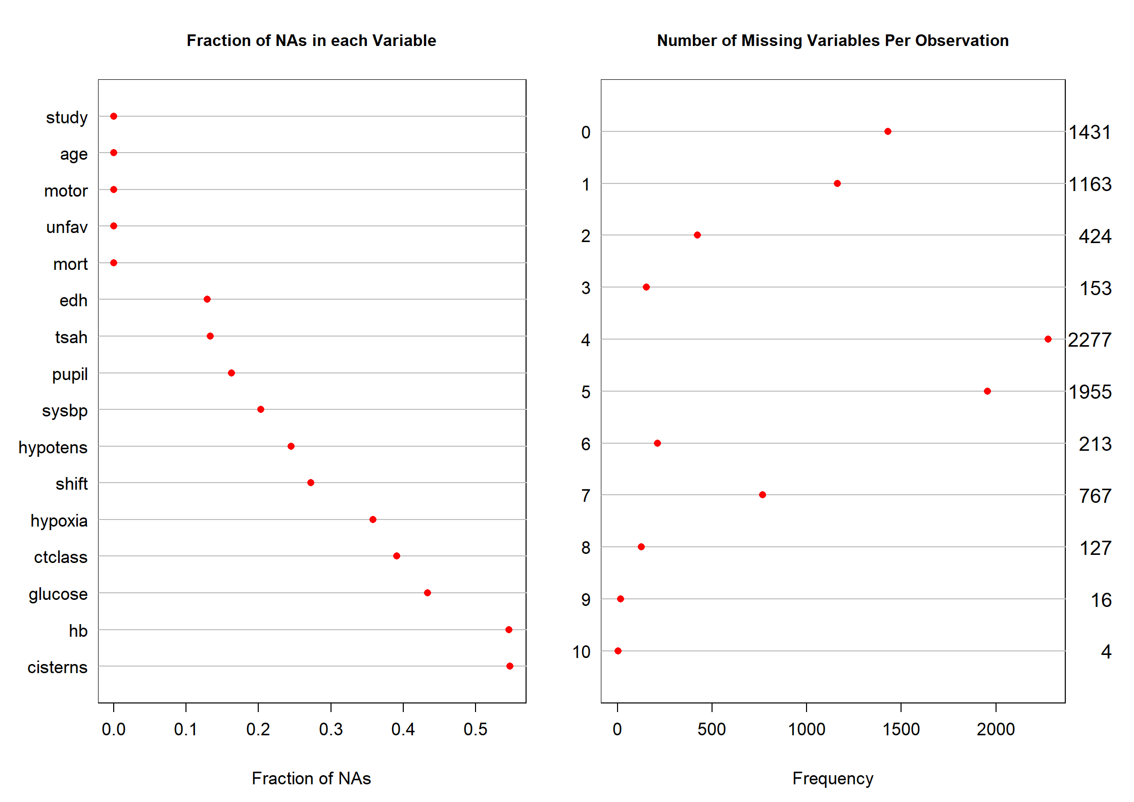
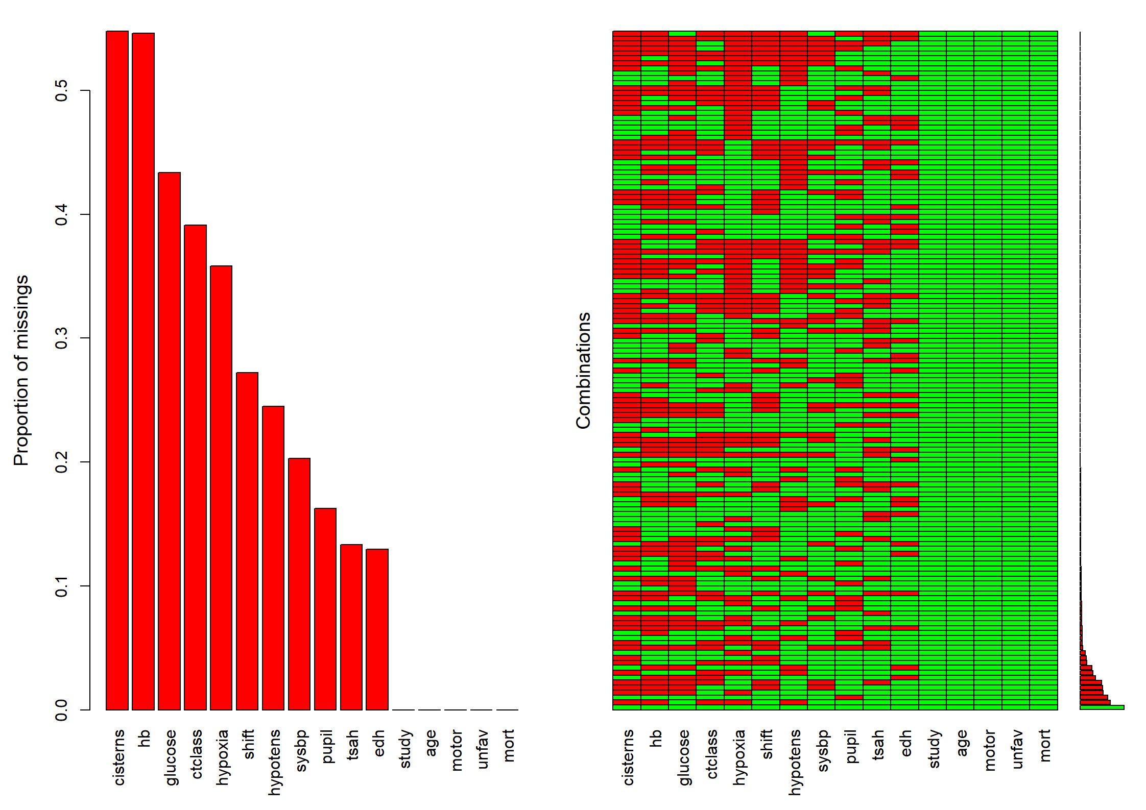
md.pattern(dMNAR)
na.pattern(dMNAR)
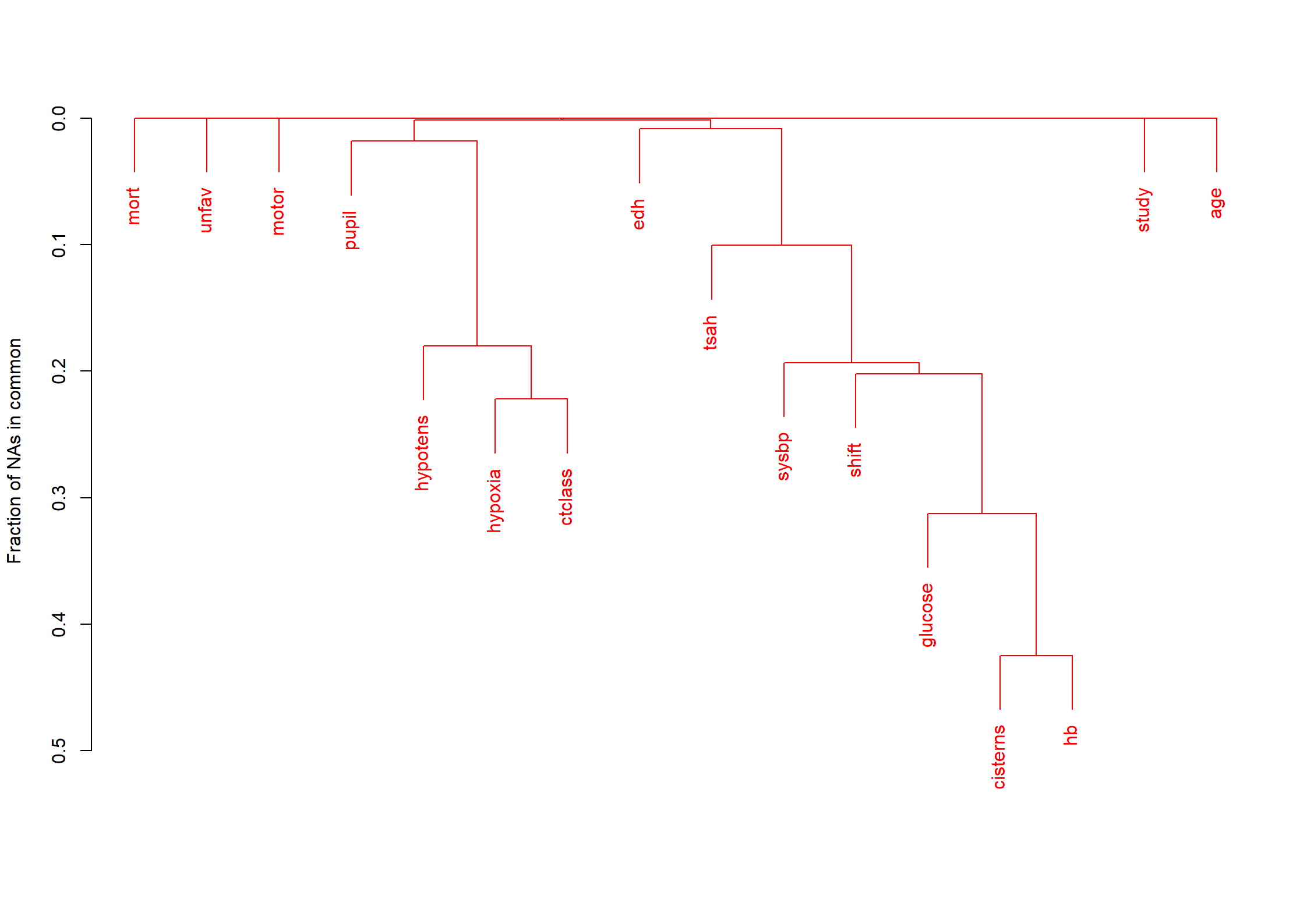
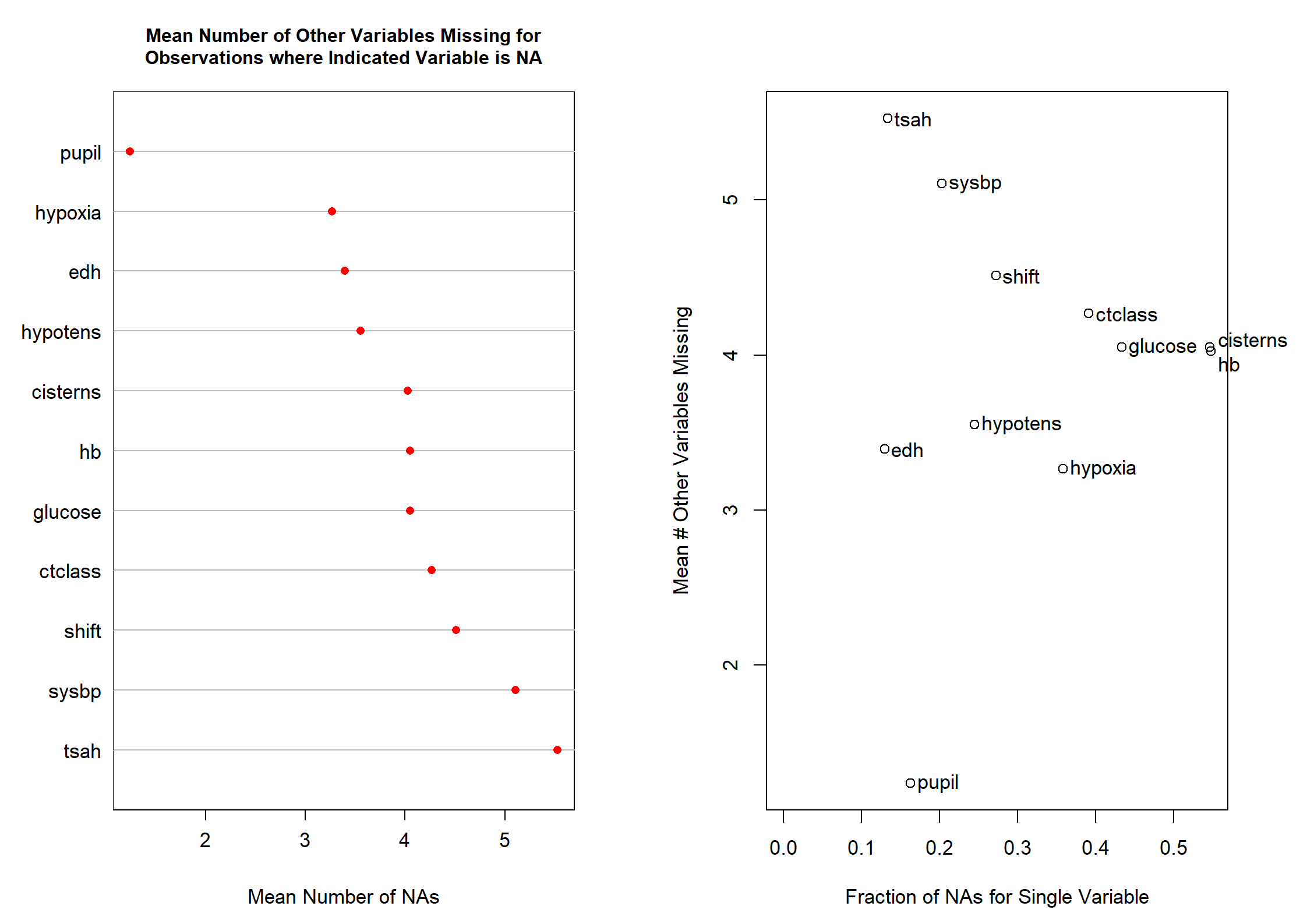
naclus(dMNAR)

set.seed(1) # For identical results at repetition
n <- 100000 # arbitrary sample size
x2 <- rnorm(n = n, mean = 0, sd = 1) # x2 standard normal
x1 <- rnorm(n = n, mean = 0, sd = 1) # Uncorrelated x1
y1.bin <- rbinom(n, 1, plogis(1 * x1 + 1 * x2)) # generate y
x1MCAR <- ifelse(runif(n) < .5, x1, NA) # MCAR mechanism for 50% of x1
x1MARx <- ifelse(rnorm(n = n, sd = .8) < x2, x1, NA) # MAR on x2, R2 50%, 50% missing (since mean x2==0)
x1MARy <- ifelse(rbinom(n, 1, .8 * y1.bin) == 1 | rbinom(n, 1, .2 * (1 - y1.bin)) == 1, NA, x1) # MAR on y, R2 50%, 50% missing (since mean y1==0)
x1MNAR <- ifelse(rnorm(n = n, sd = .8) < x1, x1, NA) # MNAR on x1, R2 50%, 50% missing (since mean x1==0)

mean(is.na(x1MARy)[y1.bin == 0])
mean(is.na(x1MARy)[y1.bin == 1])

lrm(y1.bin ~ x1 + x2)
lrm(y1.bin ~ x1MCAR + x2)
lrm(y1.bin ~ x1MARx + x2)
lrm(y1.bin ~ x1MARy + x2)
lrm(y1.bin ~ x1MNAR + x2)

# Compare fits in the various selections
fx1.CC <- lrm(y1.bin ~ x1 + x2)
fx1MARx.CC <- lrm(y1.bin ~ x1MARx + x2)
fx1MARy.CC <- lrm(y1.bin ~ x1MARy + x2)
fx1MNAR.CC <- lrm(y1.bin ~ x1MNAR + x2)

# Regression coefficients
print(rbind(
  coef(fx1.CC), coef(fx1MARx.CC),
  coef(fx1MARy.CC), coef(fx1MNAR.CC)
), digits = 3)

print(rbind(
  sqrt(diag(fx1.CC$var)), sqrt(diag(fx1MARx.CC$var)),
  sqrt(diag(fx1MARy.CC$var)), sqrt(diag(fx1MNAR.CC$var))
), digits = 3)

# Imputation; make data sets with different types of missings
d <- as.data.frame(cbind(y1.bin, x1, x2, x1MCAR, x1MARx, x1MARy, x1MNAR))
dMCAR <- d[, c(1, 3, 4)] # data set with x1 missings according to MCAR
dMARx <- d[, c(1, 3, 5)] # x1 MAR on x2
dMARy <- d[, c(1, 3, 6)] # x1 MAR on y
dMNAR <- d[, c(1, 3, 7)] # x1 MNAR at x1

## MI using the aregImpute function from rms
## help(areImpute) for more info
g <- aregImpute(~ y1.bin + x1MCAR + x2, n.impute = 5, data = d, pr = F, type = "pmm")
## fit models per imputed set and combine results using Rubin's rules
## Use fit.mult.impute() function from rms
fx1MCAR.MI <- fit.mult.impute(y1.bin ~ x1MCAR + x2, lrm, xtrans = g, data = d, pr = F)

g <- aregImpute(~ y1.bin + x1MARx + x2, n.impute = 5, data = d, pr = F, type = "pmm")
fx1MARx.MI <- fit.mult.impute(y1.bin ~ x1MARx + x2, lrm, xtrans = g, data = d, pr = F) ## areg

g <- aregImpute(~ y1.bin + x1MARy + x2, n.impute = 5, data = d, pr = F, type = "pmm")
fx1MARy.MI <- fit.mult.impute(y1.bin ~ x1MARy + x2, lrm, xtrans = g, data = d, pr = F) ## areg

g <- aregImpute(~ y1.bin + x1MNAR + x2, n.impute = 5, data = d, pr = F, type = "pmm")
fx1MNAR.MI <- fit.mult.impute(y1.bin ~ x1MNAR + x2, lrm, xtrans = g, data = d, pr = F) ## areg

# Regression coefficients after MI with aregImpute
print(rbind(
  coef(fx1MCAR.MI), coef(fx1MARx.MI),
  coef(fx1MARy.MI), coef(fx1MNAR.MI)
), digits = 3)

print(rbind(
  sqrt(diag(fx1MCAR.MI$var)), sqrt(diag(fx1MARx.MI$var)),
  sqrt(diag(fx1MARy.MI$var)), sqrt(diag(fx1MNAR.MI$var))
), digits = 3)