8 Case Study on Dealing with Missing Values

Read and describe data file

Code show/hide

TBI1 <- read.csv("data/TBI1.csv", row.names = 1)
TBI1$study <- as.factor(TBI1$study)
TBI1$pupil <- as.factor(TBI1$pupil)
TBI1$ctclass <- as.factor(TBI1$ctclass)
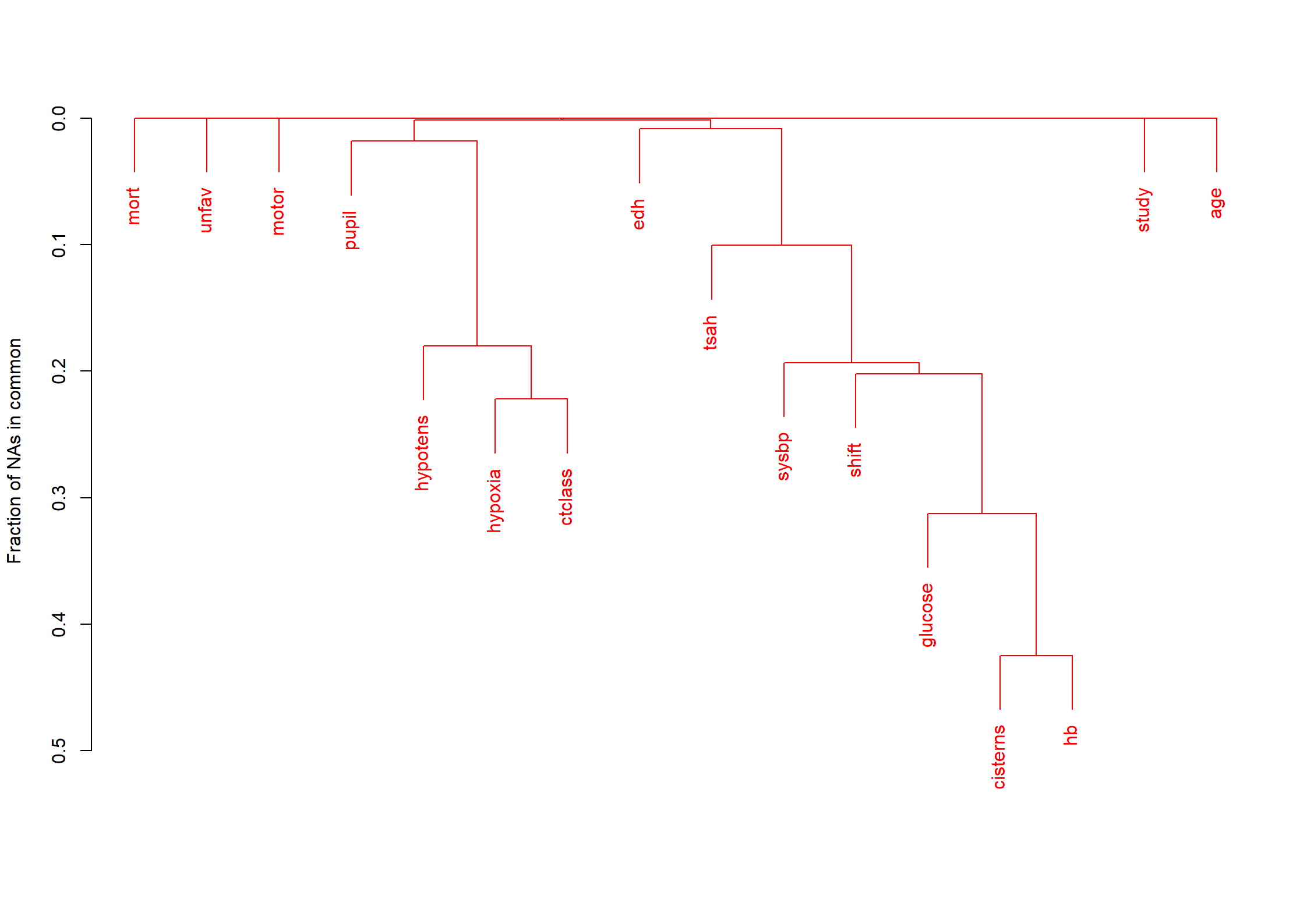
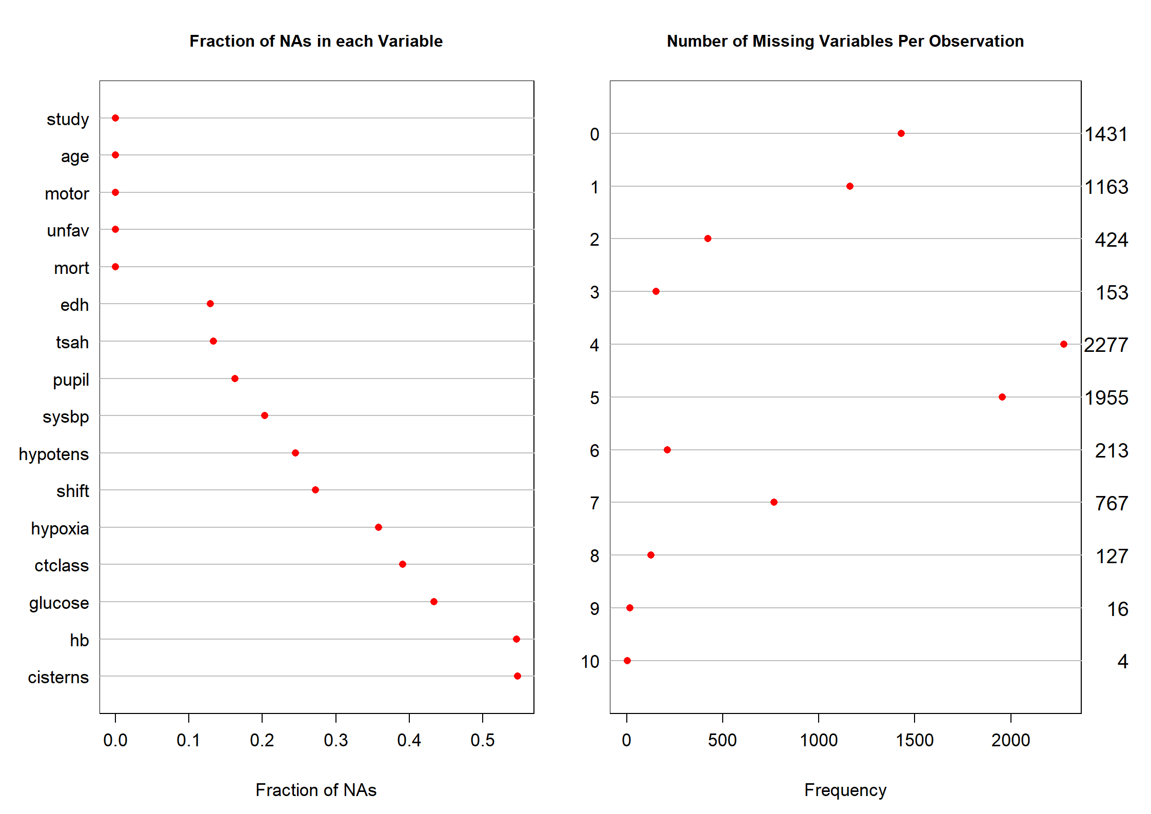
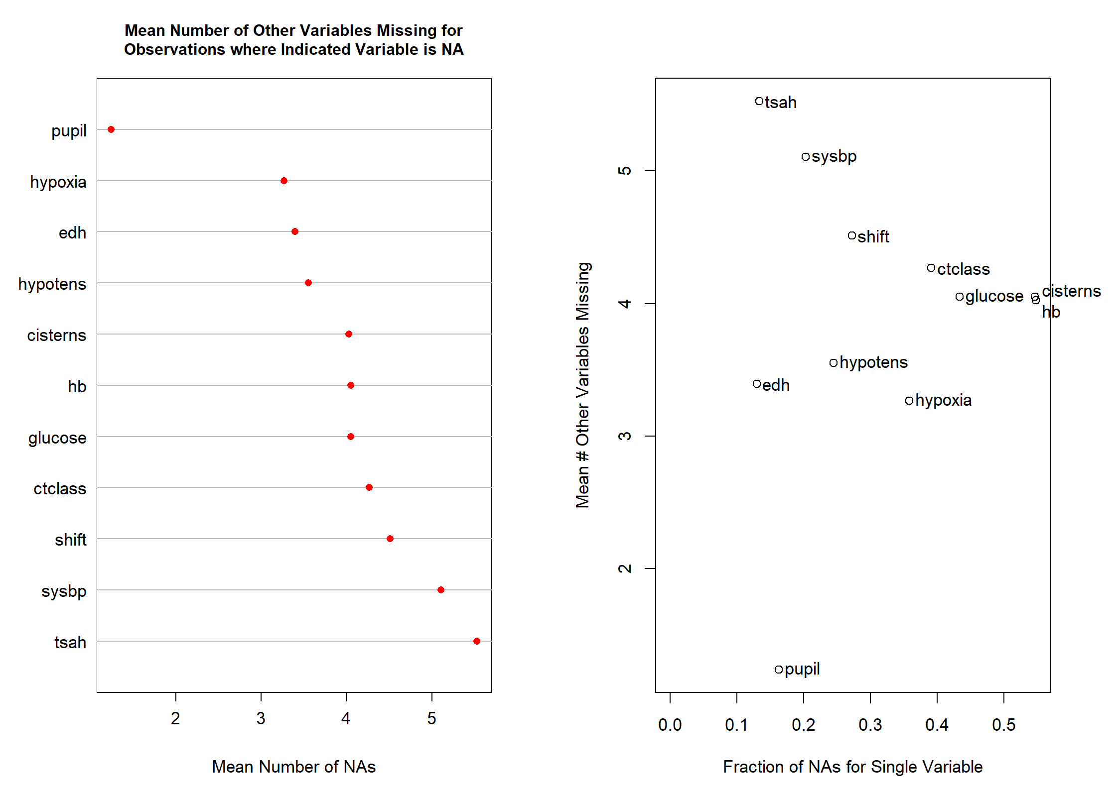
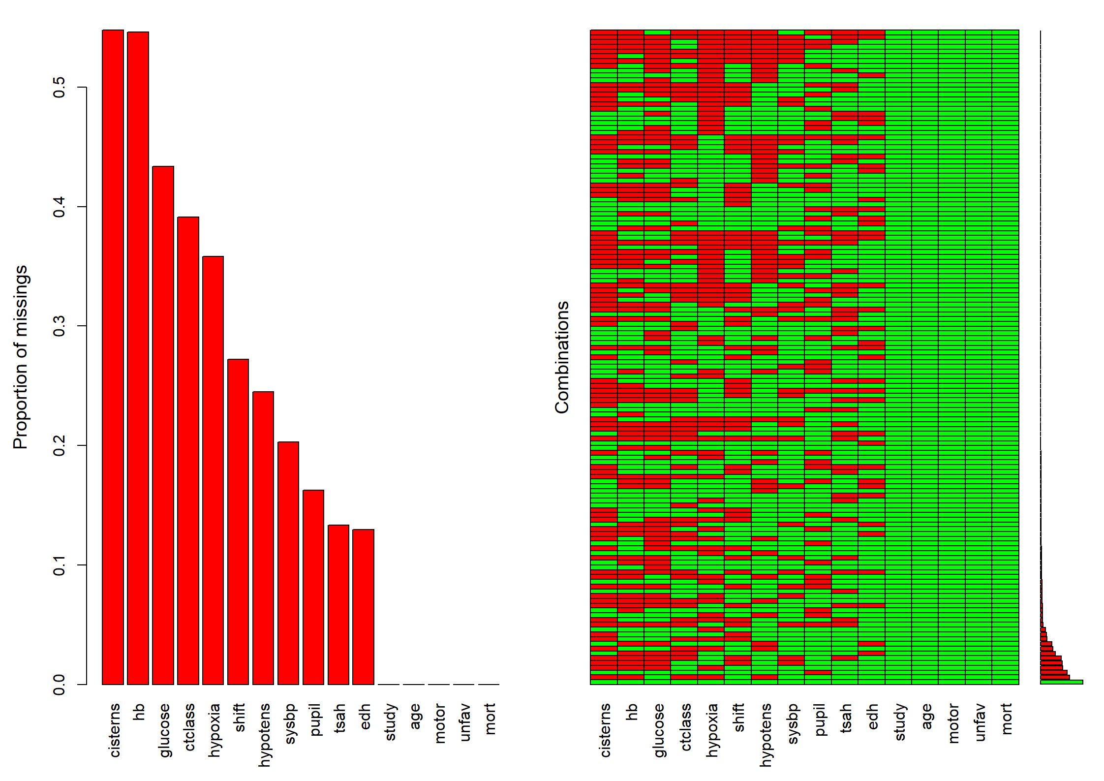
describe(TBI1)

TBI1 

 16  Variables      8530  Observations
----------------------------------------------------------------------------------------------------
study 
       n  missing distinct 
    8530        0       11 
                                                                            
Value          1     2     3     4     5     6     7     8     9    10    11
Frequency   1118  1041   409   919  1510   350   812   604   126   822   819
Proportion 0.131 0.122 0.048 0.108 0.177 0.041 0.095 0.071 0.015 0.096 0.096
----------------------------------------------------------------------------------------------------
age 
       n  missing distinct     Info     Mean      Gmd      .05      .10      .25      .50      .75 
    8530        0       80    0.999     34.7    17.59       17       18       21       30       45 
     .90      .95 
      59       65 

lowest : 14 15 16 17 18, highest: 89 90 91 92 93
----------------------------------------------------------------------------------------------------
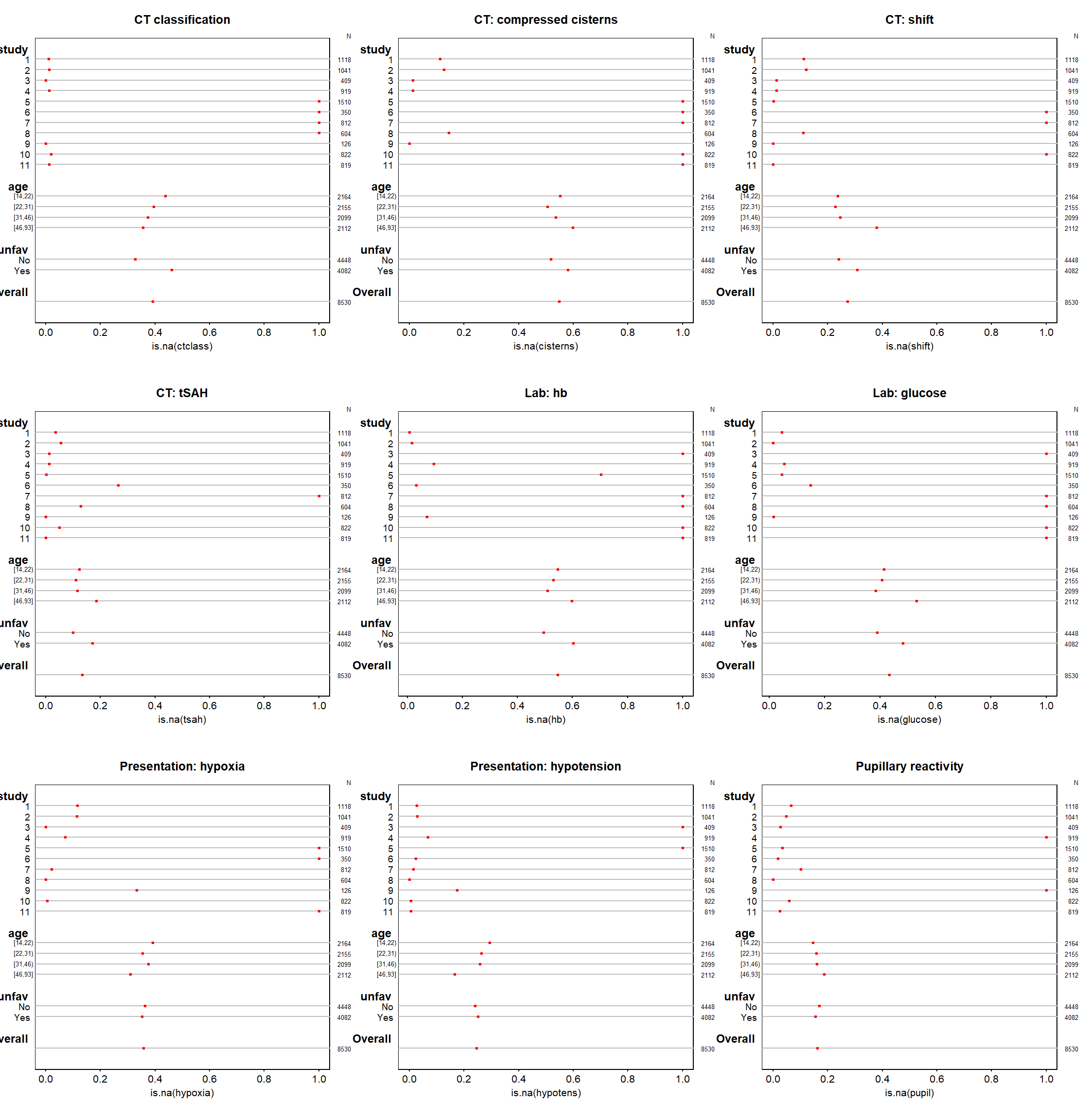
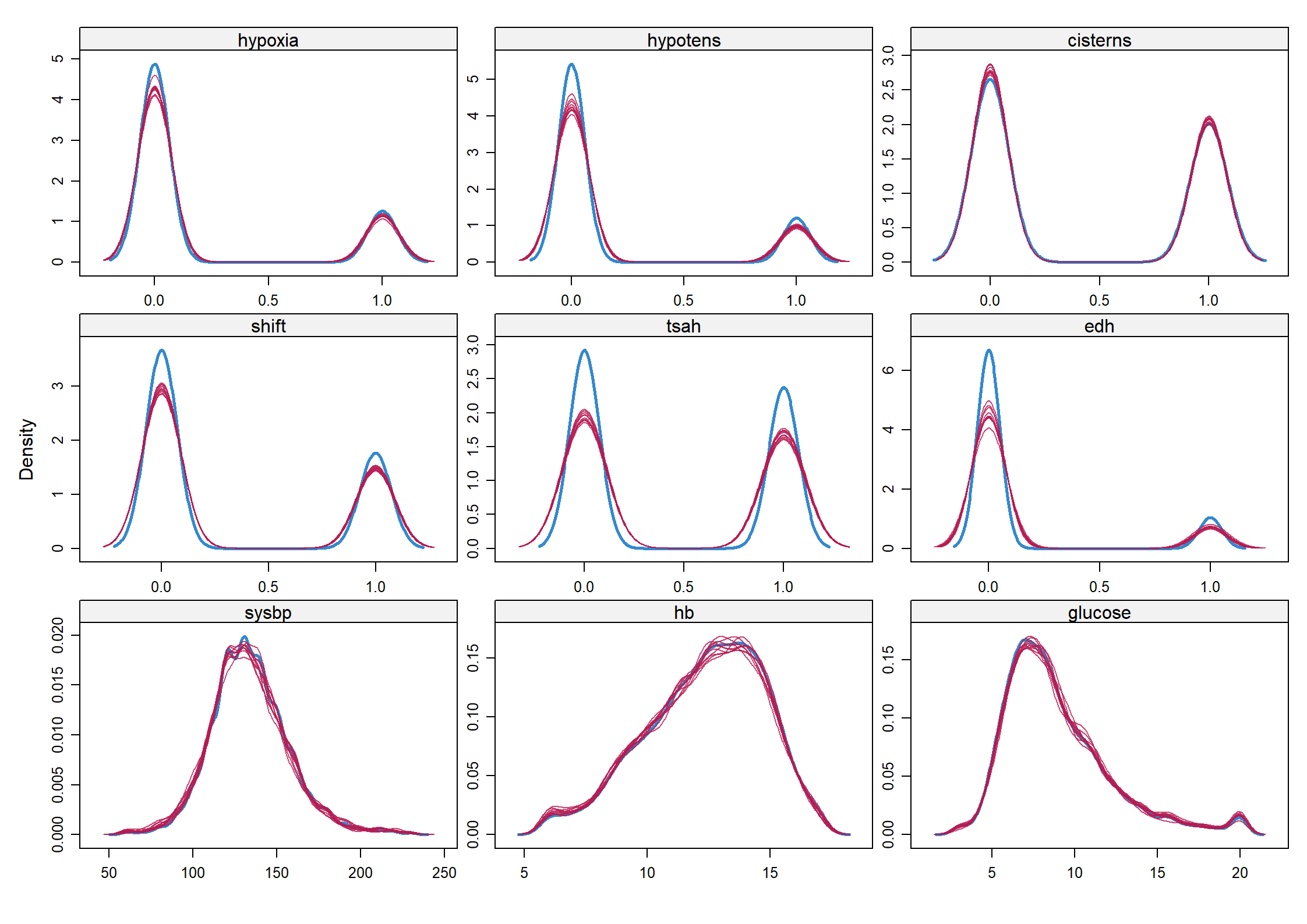
hypoxia 
       n  missing distinct     Info      Sum     Mean      Gmd 
    5473     3057        2    0.489     1122    0.205    0.326 

----------------------------------------------------------------------------------------------------
hypotens 
       n  missing distinct     Info      Sum     Mean      Gmd 
    6440     2090        2    0.447     1173   0.1821    0.298 

----------------------------------------------------------------------------------------------------
cisterns 
       n  missing distinct     Info      Sum     Mean      Gmd 
    3857     4673        2    0.736     1661   0.4306   0.4905 

----------------------------------------------------------------------------------------------------
shift 
       n  missing distinct     Info      Sum     Mean      Gmd 
    6209     2321        2    0.658     2020   0.3253   0.4391 

----------------------------------------------------------------------------------------------------
tsah 
       n  missing distinct     Info      Sum     Mean      Gmd 
    7393     1137        2    0.742     3313   0.4481   0.4947 

----------------------------------------------------------------------------------------------------
edh 
       n  missing distinct     Info      Sum     Mean      Gmd 
    7425     1105        2     0.35     1001   0.1348   0.2333 

----------------------------------------------------------------------------------------------------
pupil 
       n  missing distinct 
    7143     1387        3 
                            
Value          1     2     3
Frequency   4498   887  1758
Proportion 0.630 0.124 0.246
----------------------------------------------------------------------------------------------------
motor 
       n  missing distinct 
    8530        0        5 
                                        
Value        1/2     3     4   5/6     9
Frequency   2439  1085  1941  2602   463
Proportion 0.286 0.127 0.228 0.305 0.054
----------------------------------------------------------------------------------------------------
ctclass 
       n  missing distinct 
    5192     3338        3 
                            
Value          1     2     3
Frequency   2198  1050  1944
Proportion 0.423 0.202 0.374
----------------------------------------------------------------------------------------------------
sysbp 
       n  missing distinct     Info     Mean      Gmd      .05      .10      .25      .50      .75 
    6797     1733     1653    0.999    134.3     25.3      100      108      120      132      148 
     .90      .95 
     162      175 

lowest : 60    62    64    64.19 65.6 , highest: 219   220   222   226   230  
----------------------------------------------------------------------------------------------------
hb 
       n  missing distinct     Info     Mean      Gmd      .05      .10      .25      .50      .75 
    3871     4659      195        1    12.39    2.685      8.1      9.1     10.8     12.6     14.2 
     .90      .95 
    15.2     15.8 

lowest : 6       6.1     6.12311 6.2     6.28424, highest: 16.7    16.79   16.8    16.9    17     
----------------------------------------------------------------------------------------------------
glucose 
       n  missing distinct     Info     Mean      Gmd      .05      .10      .25      .50      .75 
    4830     3700      706        1    8.894    3.393    5.100    5.611    6.700    8.200   10.400 
     .90      .95 
  13.091   15.500 

lowest : 3       3.03    3.05556 3.2     3.3    , highest: 19.7778 19.8    19.855  19.9    20     
----------------------------------------------------------------------------------------------------
unfav 
       n  missing distinct     Info      Sum     Mean      Gmd 
    8530        0        2    0.749     4082   0.4785   0.4991 

----------------------------------------------------------------------------------------------------
mort 
       n  missing distinct     Info      Sum     Mean      Gmd 
    8530        0        2    0.606     2396   0.2809    0.404 

----------------------------------------------------------------------------------------------------

Missing value analysis

Start with rms functions

Code show/hide

na.patterns <- naclus(TBI1)
plot(na.patterns, ylab = "Fraction of NAs in common", col = "red")

Code show/hide

par(mfrow = c(1, 2))
naplot(na.patterns, col = "red", cex = 1.1, cex.main = 0.9)

Other visualization: VIM package

Code show/hide

library(VIM)
par(mfrow = c(1, 1))
aggr(TBI1, sortVars = T, col = c("green", "red"))


 Variables sorted by number of missings: 
 Variable     Count
 cisterns 0.5478312
       hb 0.5461899
  glucose 0.4337632
  ctclass 0.3913247
  hypoxia 0.3583822
    shift 0.2720985
 hypotens 0.2450176
    sysbp 0.2031653
    pupil 0.1626026
     tsah 0.1332943
      edh 0.1295428
    study 0.0000000
      age 0.0000000
    motor 0.0000000
    unfav 0.0000000
     mort 0.0000000

9 separate plots

Code show/hide

par(mar = c(4, 4, 3, 1) + 0.1,mfrow = c(3, 3))

plot(summary(is.na(ctclass) ~ study + age + unfav, data = TBI1), main = "CT classification", pch = 19, cex.main = 0.6, cex.axis = 0.8, cex.lab = .6, cex.sub = 0.3, col = "red",reset.par = FALSE)

plot(summary(is.na(cisterns) ~ study + age + unfav, data = TBI1), main = "CT: compressed cisterns", pch = 19, cex.main = 0.6, cex.axis = 0.8, cex.lab = .6, cex.sub = 0.3, col = "red",reset.par = FALSE)

plot(summary(is.na(shift) ~ study + age + unfav, data = TBI1), main = "CT: shift", pch = 19, cex.main = 0.6, cex.axis = 0.8, cex.lab = .6, cex.sub = 0.3, col = "red",reset.par = FALSE)

plot(summary(is.na(tsah) ~ study + age + unfav, data = TBI1), main = "CT: tSAH", pch = 19, cex.main = 0.6, cex.axis = 0.8, cex.lab = .6, cex.sub = 0.3, col = "red",reset.par = FALSE)

plot(summary(is.na(hb) ~ study + age + unfav, data = TBI1), main = "Lab: hb", pch = 19, cex.main = 0.6, cex.axis = 0.8, cex.lab = .6, cex.sub = 0.3, col = "red",reset.par = FALSE)

plot(summary(is.na(glucose) ~ study + age + unfav, data = TBI1), main = "Lab: glucose", pch = 19, cex.main = 0.6, cex.axis = 0.8, cex.lab = .6, cex.sub = 0.3, col = "red",reset.par = FALSE)

plot(summary(is.na(hypoxia) ~ study + age + unfav, data = TBI1), main = "Presentation: hypoxia", pch = 19, cex.main = 0.6, cex.axis = 0.8, cex.lab = .6, cex.sub = 0.3, col = "red",reset.par = FALSE)

plot(summary(is.na(hypotens) ~ study + age + unfav, data = TBI1), main = "Presentation: hypotension", pch = 19, cex.main = 0.6, cex.axis = 0.8, cex.lab = .6, cex.sub = 0.3, col = "red",reset.par = FALSE)

plot(summary(is.na(pupil) ~ study + age + unfav, data = TBI1), main = "Pupillary reactivity", pch = 19, cex.main = 0.6, cex.axis = 0.8, cex.lab = .6, cex.sub = 0.3, col = "red",reset.par = FALSE)

Code show/hide

# End plot missing patterns

Imputation

mice in action

We define the matrix pmat for mice predictorMatrix.
A value of ‘1’ means that the column variable is used as a predictor for the target variable (in the rows). The diagonal of ‘predictorMatrix’ must be zero. In our matrix we don’t want ‘study’, ‘age’, ‘motor’, ‘unfav’ and ‘mort’ to be imputed.

Code show/hide

p <- 16
pmat <- matrix(rep(1, p * p), nrow = p, ncol = p)
diag(pmat) <- rep(0, p)
pmat[, c(1:2, 10, 15:16)] <- 0 # set some columns to zero
pmat[c(1:2, 10, 15:16), ] <- 0 # set the rows for the same variables to zero

## defines data to be used and the imputation method for each column, seed=1
gm <- mice(TBI1,
  m = 10,
  imputationMethod = c(
    "polyreg", "pmm", "logreg", "logreg", "logreg", "logreg", "logreg", "logreg", "polyreg",
    "polyreg", "polyreg", "pmm", "pmm", "pmm", "logreg", "logreg"
  ), predictorMatrix = pmat, seed = 1
)


 iter imp variable
  1   1  hypoxia  hypotens  cisterns  shift  tsah  edh  pupil  ctclass  sysbp  hb  glucose
  1   2  hypoxia  hypotens  cisterns  shift  tsah  edh  pupil  ctclass  sysbp  hb  glucose
  1   3  hypoxia  hypotens  cisterns  shift  tsah  edh  pupil  ctclass  sysbp  hb  glucose
  1   4  hypoxia  hypotens  cisterns  shift  tsah  edh  pupil  ctclass  sysbp  hb  glucose
  1   5  hypoxia  hypotens  cisterns  shift  tsah  edh  pupil  ctclass  sysbp  hb  glucose
  1   6  hypoxia  hypotens  cisterns  shift  tsah  edh  pupil  ctclass  sysbp  hb  glucose
  1   7  hypoxia  hypotens  cisterns  shift  tsah  edh  pupil  ctclass  sysbp  hb  glucose
  1   8  hypoxia  hypotens  cisterns  shift  tsah  edh  pupil  ctclass  sysbp  hb  glucose
  1   9  hypoxia  hypotens  cisterns  shift  tsah  edh  pupil  ctclass  sysbp  hb  glucose
  1   10  hypoxia  hypotens  cisterns  shift  tsah  edh  pupil  ctclass  sysbp  hb  glucose
  2   1  hypoxia  hypotens  cisterns  shift  tsah  edh  pupil  ctclass  sysbp  hb  glucose
  2   2  hypoxia  hypotens  cisterns  shift  tsah  edh  pupil  ctclass  sysbp  hb  glucose
  2   3  hypoxia  hypotens  cisterns  shift  tsah  edh  pupil  ctclass  sysbp  hb  glucose
  2   4  hypoxia  hypotens  cisterns  shift  tsah  edh  pupil  ctclass  sysbp  hb  glucose
  2   5  hypoxia  hypotens  cisterns  shift  tsah  edh  pupil  ctclass  sysbp  hb  glucose
  2   6  hypoxia  hypotens  cisterns  shift  tsah  edh  pupil  ctclass  sysbp  hb  glucose
  2   7  hypoxia  hypotens  cisterns  shift  tsah  edh  pupil  ctclass  sysbp  hb  glucose
  2   8  hypoxia  hypotens  cisterns  shift  tsah  edh  pupil  ctclass  sysbp  hb  glucose
  2   9  hypoxia  hypotens  cisterns  shift  tsah  edh  pupil  ctclass  sysbp  hb  glucose
  2   10  hypoxia  hypotens  cisterns  shift  tsah  edh  pupil  ctclass  sysbp  hb  glucose
  3   1  hypoxia  hypotens  cisterns  shift  tsah  edh  pupil  ctclass  sysbp  hb  glucose
  3   2  hypoxia  hypotens  cisterns  shift  tsah  edh  pupil  ctclass  sysbp  hb  glucose
  3   3  hypoxia  hypotens  cisterns  shift  tsah  edh  pupil  ctclass  sysbp  hb  glucose
  3   4  hypoxia  hypotens  cisterns  shift  tsah  edh  pupil  ctclass  sysbp  hb  glucose
  3   5  hypoxia  hypotens  cisterns  shift  tsah  edh  pupil  ctclass  sysbp  hb  glucose
  3   6  hypoxia  hypotens  cisterns  shift  tsah  edh  pupil  ctclass  sysbp  hb  glucose
  3   7  hypoxia  hypotens  cisterns  shift  tsah  edh  pupil  ctclass  sysbp  hb  glucose
  3   8  hypoxia  hypotens  cisterns  shift  tsah  edh  pupil  ctclass  sysbp  hb  glucose
  3   9  hypoxia  hypotens  cisterns  shift  tsah  edh  pupil  ctclass  sysbp  hb  glucose
  3   10  hypoxia  hypotens  cisterns  shift  tsah  edh  pupil  ctclass  sysbp  hb  glucose
  4   1  hypoxia  hypotens  cisterns  shift  tsah  edh  pupil  ctclass  sysbp  hb  glucose
  4   2  hypoxia  hypotens  cisterns  shift  tsah  edh  pupil  ctclass  sysbp  hb  glucose
  4   3  hypoxia  hypotens  cisterns  shift  tsah  edh  pupil  ctclass  sysbp  hb  glucose
  4   4  hypoxia  hypotens  cisterns  shift  tsah  edh  pupil  ctclass  sysbp  hb  glucose
  4   5  hypoxia  hypotens  cisterns  shift  tsah  edh  pupil  ctclass  sysbp  hb  glucose
  4   6  hypoxia  hypotens  cisterns  shift  tsah  edh  pupil  ctclass  sysbp  hb  glucose
  4   7  hypoxia  hypotens  cisterns  shift  tsah  edh  pupil  ctclass  sysbp  hb  glucose
  4   8  hypoxia  hypotens  cisterns  shift  tsah  edh  pupil  ctclass  sysbp  hb  glucose
  4   9  hypoxia  hypotens  cisterns  shift  tsah  edh  pupil  ctclass  sysbp  hb  glucose
  4   10  hypoxia  hypotens  cisterns  shift  tsah  edh  pupil  ctclass  sysbp  hb  glucose
  5   1  hypoxia  hypotens  cisterns  shift  tsah  edh  pupil  ctclass  sysbp  hb  glucose
  5   2  hypoxia  hypotens  cisterns  shift  tsah  edh  pupil  ctclass  sysbp  hb  glucose
  5   3  hypoxia  hypotens  cisterns  shift  tsah  edh  pupil  ctclass  sysbp  hb  glucose
  5   4  hypoxia  hypotens  cisterns  shift  tsah  edh  pupil  ctclass  sysbp  hb  glucose
  5   5  hypoxia  hypotens  cisterns  shift  tsah  edh  pupil  ctclass  sysbp  hb  glucose
  5   6  hypoxia  hypotens  cisterns  shift  tsah  edh  pupil  ctclass  sysbp  hb  glucose
  5   7  hypoxia  hypotens  cisterns  shift  tsah  edh  pupil  ctclass  sysbp  hb  glucose
  5   8  hypoxia  hypotens  cisterns  shift  tsah  edh  pupil  ctclass  sysbp  hb  glucose
  5   9  hypoxia  hypotens  cisterns  shift  tsah  edh  pupil  ctclass  sysbp  hb  glucose
  5   10  hypoxia  hypotens  cisterns  shift  tsah  edh  pupil  ctclass  sysbp  hb  glucose

Code show/hide

gm

Class: mids
Number of multiple imputations:  10 
Imputation methods:
    study       age   hypoxia  hypotens  cisterns     shift      tsah       edh     pupil     motor 
       ""        ""     "pmm"     "pmm"     "pmm"     "pmm"     "pmm"     "pmm" "polyreg"        "" 
  ctclass     sysbp        hb   glucose     unfav      mort 
"polyreg"     "pmm"     "pmm"     "pmm"        ""        "" 
PredictorMatrix:
         study age hypoxia hypotens cisterns shift tsah edh pupil motor ctclass sysbp hb glucose
study        0   0       0        0        0     0    0   0     0     0       0     0  0       0
age          0   0       0        0        0     0    0   0     0     0       0     0  0       0
hypoxia      0   0       0        1        1     1    1   1     1     0       1     1  1       1
hypotens     0   0       1        0        1     1    1   1     1     0       1     1  1       1
cisterns     0   0       1        1        0     1    1   1     1     0       1     1  1       1
shift        0   0       1        1        1     0    1   1     1     0       1     1  1       1
         unfav mort
study        0    0
age          0    0
hypoxia      0    0
hypotens     0    0
cisterns     0    0
shift        0    0

Code show/hide

densityplot(gm) # Nice check for imputed vs original distributions

Univariate, CC analyses for age and motor

Code show/hide

lrm(unfav ~ study + age, data = TBI1)

Logistic Regression Model

lrm(formula = unfav ~ study + age, data = TBI1)

                       Model Likelihood        Discrimination    Rank Discrim.    
                             Ratio Test               Indexes          Indexes    
Obs          8530    LR chi2     746.50        R2       0.112    C       0.660    
 0           4448    d.f.            11      R2(11,8530)0.083    Dxy     0.320    
 1           4082    Pr(> chi2) <0.0001    R2(11,6385.7)0.109    gamma   0.321    
max |deriv| 3e-09                              Brier    0.229    tau-a   0.160    

          Coef    S.E.   Wald Z Pr(>|Z|)
Intercept -1.4648 0.0817 -17.93 <0.0001 
study=2   -0.0930 0.0902  -1.03 0.3028  
study=3    0.1502 0.1197   1.26 0.2094  
study=4   -0.0521 0.0932  -0.56 0.5757  
study=5    0.5481 0.0819   6.69 <0.0001 
study=6    0.2838 0.1266   2.24 0.0249  
study=7    0.8219 0.0983   8.36 <0.0001 
study=8    1.0808 0.1076  10.04 <0.0001 
study=9    0.7223 0.1934   3.73 0.0002  
study=10   0.1961 0.0967   2.03 0.0425  
study=11  -0.1226 0.0966  -1.27 0.2043  
age        0.0320 0.0015  20.91 <0.0001

Code show/hide

lrm(unfav ~ study + motor, data = TBI1)

Logistic Regression Model

lrm(formula = unfav ~ study + motor, data = TBI1)

                       Model Likelihood        Discrimination    Rank Discrim.    
                             Ratio Test               Indexes          Indexes    
Obs          8530    LR chi2    1259.58        R2       0.183    C       0.715    
 0           4448    d.f.            14      R2(14,8530)0.136    Dxy     0.429    
 1           4082    Pr(> chi2) <0.0001    R2(14,6385.7)0.177    gamma   0.441    
max |deriv| 1e-09                              Brier    0.214    tau-a   0.214    

          Coef    S.E.   Wald Z Pr(>|Z|)
Intercept  0.7308 0.0802   9.11 <0.0001 
study=2   -0.0444 0.0933  -0.48 0.6339  
study=3    0.0694 0.1231   0.56 0.5728  
study=4   -0.1932 0.0966  -2.00 0.0455  
study=5    0.0684 0.0863   0.79 0.4279  
study=6   -0.1149 0.1325  -0.87 0.3856  
study=7    0.9001 0.1048   8.59 <0.0001 
study=8    0.7259 0.1120   6.48 <0.0001 
study=9    0.1781 0.2024   0.88 0.3788  
study=10   0.3329 0.1015   3.28 0.0010  
study=11  -0.3365 0.1008  -3.34 0.0008  
motor=3   -0.4900 0.0781  -6.27 <0.0001 
motor=4   -1.1764 0.0662 -17.77 <0.0001 
motor=5/6 -1.8656 0.0653 -28.57 <0.0001 
motor=9   -0.9513 0.1137  -8.36 <0.0001

Prediction model analyses

Code show/hide

## CC, n = 2428
lrm(unfav ~ study + age + motor + pupil + hypoxia + hypotens + ctclass + tsah, data = TBI1)
## SI, n = 8530
lrm(unfav ~ study + age + motor + pupil + hypoxia + hypotens + ctclass + tsah, data = complete(gm, action = 1))
## MI, n = 8530
fit.mult.impute(unfav ~ study + age + motor + pupil + hypoxia + hypotens + ctclass + tsah, lrm, xtrans = gm, data = TBI1)

Make adjusted analyses per complete predictor

Code show/hide

names.uni <- Cs(pupil, hypoxia, hypotens, ctclass, tsah) # 5 names
TBIc <- complete(gm, action = "long", include = TRUE) # completed data set

###################################################
# pupils
TBI2 <- TBIc[!TBIc$.id %in% TBIc$.id[is.na(TBIc$pupil)], ]
gm2 <- as.mids(TBI2)
fit.CC <- lrm(unfav ~ study + pupil, data = TBI2[TBI2$.imp == 0, ])
fit.SI <- lrm(unfav ~ study + age + motor + pupil + hypoxia + hypotens + ctclass + tsah, data = TBI2[TBI2$.imp == 1, ])
fit.MI <- fit.mult.impute(unfav ~ study + age + motor + pupil + hypoxia + hypotens + ctclass + tsah, lrm, xtrans = gm2)

Code show/hide

options(digits = 2)
i <- 1 # indicates index for the predictor we are studying
print(coef(fit.CC)[startsWith(names(coef(fit.CC)), names.uni[i])]) # CC
print(sqrt(diag(fit.CC$var))[startsWith(names(coef(fit.CC)), names.uni[i])])
print(coef(fit.SI)[startsWith(names(coef(fit.SI)), names.uni[i])]) # SI
print(sqrt(diag(fit.SI$var))[startsWith(names(coef(fit.SI)), names.uni[i])])
print(coef(fit.MI)[startsWith(names(coef(fit.MI)), names.uni[i])]) # MI
print(sqrt(diag(fit.MI$var))[startsWith(names(coef(fit.MI)), names.uni[i])])

Code show/hide

# hypoxia
TBI2 <- TBIc[!TBIc$.id %in% TBIc$.id[is.na(TBIc$hypoxia)], ]
gm2 <- as.mids(TBI2)
fit.CC <- lrm(unfav ~ study + hypoxia, data = TBI2[TBI2$.imp == 0, ])
fit.SI <- lrm(unfav ~ study + age + motor + pupil + hypoxia + hypotens + ctclass + tsah, data = TBI2[TBI2$.imp == 1, ])
fit.MI <- fit.mult.impute(unfav ~ study + age + motor + pupil + hypoxia + hypotens + ctclass + tsah, lrm, xtrans = gm2)

i <- 2 # index 2
print(coef(fit.CC)[startsWith(names(coef(fit.CC)), names.uni[i])]) # CC
print(sqrt(diag(fit.CC$var))[startsWith(names(coef(fit.CC)), names.uni[i])])
print(coef(fit.SI)[startsWith(names(coef(fit.SI)), names.uni[i])]) # SI
print(sqrt(diag(fit.SI$var))[startsWith(names(coef(fit.SI)), names.uni[i])])
print(coef(fit.MI)[startsWith(names(coef(fit.MI)), names.uni[i])]) # MI
print(sqrt(diag(fit.MI$var))[startsWith(names(coef(fit.MI)), names.uni[i])])

# hypotens
TBI2 <- TBIc[!TBIc$.id %in% TBIc$.id[is.na(TBIc$hypotens)], ]
gm2 <- as.mids(TBI2)
fit.CC <- lrm(unfav ~ study + hypotens, data = TBI2[TBI2$.imp == 0, ])
fit.SI <- lrm(unfav ~ study + age + motor + pupil + hypoxia + hypotens + ctclass + tsah, data = TBI2[TBI2$.imp == 1, ])
fit.MI <- fit.mult.impute(unfav ~ study + age + motor + pupil + hypoxia + hypotens + ctclass + tsah, lrm, xtrans = gm2)

i <- 3
print(coef(fit.CC)[startsWith(names(coef(fit.CC)), names.uni[i])]) # CC
print(sqrt(diag(fit.CC$var))[startsWith(names(coef(fit.CC)), names.uni[i])])
print(coef(fit.SI)[startsWith(names(coef(fit.SI)), names.uni[i])]) # SI
print(sqrt(diag(fit.SI$var))[startsWith(names(coef(fit.SI)), names.uni[i])])
print(coef(fit.MI)[startsWith(names(coef(fit.MI)), names.uni[i])]) # MI
print(sqrt(diag(fit.MI$var))[startsWith(names(coef(fit.MI)), names.uni[i])])

# ctclass
TBI2 <- TBIc[!TBIc$.id %in% TBIc$.id[is.na(TBIc$ctclass)], ]
gm2 <- as.mids(TBI2)
fit.CC <- lrm(unfav ~ study + ctclass, data = TBI2[TBI2$.imp == 0, ])
fit.SI <- lrm(unfav ~ study + age + motor + pupil + hypoxia + hypotens + ctclass + tsah, data = TBI2[TBI2$.imp == 1, ])
fit.MI <- fit.mult.impute(unfav ~ study + age + motor + pupil + hypoxia + hypotens + ctclass + tsah, lrm, xtrans = gm2)

i <- 4
print(coef(fit.CC)[startsWith(names(coef(fit.CC)), names.uni[i])]) # CC
print(sqrt(diag(fit.CC$var))[startsWith(names(coef(fit.CC)), names.uni[i])])
print(coef(fit.SI)[startsWith(names(coef(fit.SI)), names.uni[i])]) # SI
print(sqrt(diag(fit.SI$var))[startsWith(names(coef(fit.SI)), names.uni[i])])
print(coef(fit.MI)[startsWith(names(coef(fit.MI)), names.uni[i])]) # MI
print(sqrt(diag(fit.MI$var))[startsWith(names(coef(fit.MI)), names.uni[i])])

# tsah
TBI2 <- TBIc[!TBIc$.id %in% TBIc$.id[is.na(TBIc$tsah)], ]
gm2 <- as.mids(TBI2)
fit.CC <- lrm(unfav ~ study + tsah, data = TBI2[TBI2$.imp == 0, ])
fit.SI <- lrm(unfav ~ study + age + motor + pupil + hypoxia + hypotens + ctclass + tsah, data = TBI2[TBI2$.imp == 1, ])
fit.MI <- fit.mult.impute(unfav ~ study + age + motor + pupil + hypoxia + hypotens + ctclass + tsah, lrm, xtrans = gm2)

i <- 5
print(coef(fit.CC)[startsWith(names(coef(fit.CC)), names.uni[i])]) # CC
print(sqrt(diag(fit.CC$var))[startsWith(names(coef(fit.CC)), names.uni[i])])
print(coef(fit.SI)[startsWith(names(coef(fit.SI)), names.uni[i])]) # SI
print(sqrt(diag(fit.SI$var))[startsWith(names(coef(fit.SI)), names.uni[i])])
print(coef(fit.MI)[startsWith(names(coef(fit.MI)), names.uni[i])]) # MI
print(sqrt(diag(fit.MI$var))[startsWith(names(coef(fit.MI)), names.uni[i])])

## End C, SI, and MI analyses ##
################################